Chapter 6 Genotype files in practice
Learning outcomes At the end of this chapter, you will be able to recognize and describe the format of SNP genotype files.
In case you read this book from the beginning, you now have a good plan where to place your files and the support programs installed. You only need one more thing, and that is the data.
So where you can get some?
The good news is that due to journal and funding agency policies, and the general goodwill of various research teams there is a lot of SNP data available. For this introduction and also the follow-up demonstrations we will use the AdaptMap goat data set. This particular data set is linked to the publication Bertolini et al. (2018)
In this post, you will see how the genomic data looks like in a PLINK format, and how to tell its basic characteristics just by looking at it. See!!! I told you the text editors will come in handy!
Unpack the zip file you obtained from Dryad into your working directory. You should see something like this:
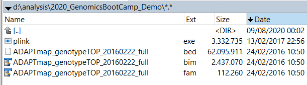
Figure 6.1: The AdaptMap goat genotype files in PLINK format
The three files contain information on animals, SNP positions, and animals in a so-called PLINK "binary ped" format. This is one of the most standard formats of the data that is efficient for computation and storage space.
Just by looking at the file names, you can see some special characteristics. The first one is that all three files have exactly the same name, and differing only in the file extension. This is on purpose. When you use the correct option in PLINK, you can refer to all three files just by using this common name, in this case, ADAPTmap_genotypeTOP_20160222_full. This is really handy!
The second thing is maybe not so apparent, but once you have seen a few data sets, it will become obvious. What I mean is that the file extensions are not just some random names, but pre-defined ones from PLINK. Also, these three belong together, and while individual files alone could give you some information, all three are needed to analyze the data.
A quick note here: technically it is possible to use any file name with the right options, but why would you complicate your life (also) with this? So I really suggest sticking to this naming convention, i.e. the same filename with .bim + .bed + .fam extensions.
So it is time to open the files! As all the file formats are described on the PLINK webpage in detail, I would point out just the main things here, and mention a few additional nuggets of information from my experience that are not easily available elsewhere.
6.1 Fam file - Info on individuals
We start with ADAPTmap_genotypeTOP_20160222_full.fam which looks like this:
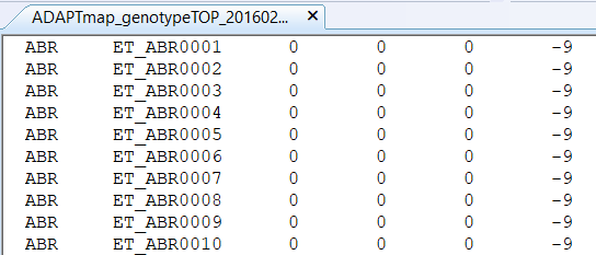
Figure 6.2: The .fam file format layout
You see that despite the funny file extension it is just a plain text file with six columns and no header. Each column has a very specific function that is described on the File formats webpage for .fam. What you need to know about the respective columns is the following:
The first column is the family identification abbreviated as FID. As the PLINK software was primarily developed for genomic analyses in humans, which is reflected in the naming terminology and default settings. In the AdaptMap data set, the use of this column is to specify breed identity. If you look into Table 1 of the linked publication, you will find that the ABR abbreviation belongs to the Abregelle goats from Ethiopia. Using the FID column to denote breed information is certainly popular, but you are not limited to it. You can use any meaningful grouping of your data as you see fit.
The second column is the "within family ID", which is just simply called "individual ID" and abbreviated as IID. Although this phrasing might suggest that the same IID could be used with different FID, it is a very good idea to have unique IIDs for each individual in your data set. For any specification of individuals within PLINK however the IID always goes together with FID, so you have to devote sufficient attention to both anyway.
and 4) The third column is the ID of the side and the fourth column the ID of the dam of the animal whose IID is denoted in the second column. If any of the parents are genotyped their ID in the third and fourth columns and their IID should correspond. It is often the case that the parents are not known, or at the time of genotyping, there is not enough time to fill out the parent information and it is set to 0. It is not a problem in most cases, but in some types of analyses, we have to be aware of this and include appropriate options (e.g. when looking at the minor allele frequency - don't worry about this now though).
Column five contains the sex information of the animal in the IID column. According to the built-in coding, 1 is for males, 2 for females, and 0 is unknown. Similar to parent information, this is also many times missing, usually not a problem, but specific options need to be included in case of any issues come up.
The sixth column is to denote the phenotype of the animal in the IID column. Because this is only a single column, only a single phenotype could be specified. In a case-control study the numerical value 1 is reserved for controls, and 2 for the cases. Alternatively, you can use any other number, including decimals for any other phenotype. In the case of missing values, you can use zero or minus nine. The question of what happens if your true phenotype measurements are 0 or -9 is still a mystery for me. In these cases, it is probably a good idea to use slightly different numbers instead.
An additional piece of information you get from the .fam files is the total number of individuals for which genotypes are available. This number is corresponding to the number of lines in the .fam file. In this case, we see that the AdaptMap data set consists of a total of 4653 genotypes!
6.2 Bim file - SNP location info
The bum file contains the locations of all SNPs in the data. When you open it with the text editor of your choice, you will see that it is nothing else than an ordinary text file called ADAPTmap_genotypeTOP_20160222_full.bim and looks like this:
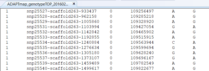
Figure 6.3: The .bim file format layout
Similar to the .fam file, the bim file has six columns, with a fixed structure described in detail on the webpage. Some info about them in brief:
The first column contains the chromosome number where the SNP is located. The goats have 29 so-called autosomal chromosomes and the number 30 is the sex chromosome. When you open a file you will see that it starts with a chromosome zero. These are the so-called unplaced SNPs, for which we know their genotype, but we are not entirely certain where they are on the genome.
The second column is the SNP name. This name is predefined during the construction of the SNP chip and fixed. If you ever want to compare versions of different SNP chips for the same species, the SNP overlaps based on their names is an excellent way to start.
The third column is the position of the SNP in Morgans or centimorgans, with zero value if you do not know or do not care. Honestly, for most of the analyses, this could be kept as zero. If you do some fancy stuff involving recombinations you can always amend this column also in existing map files.
The fourth column is the base pair coordinate of the SNP. In other words, you (well, not you personally, but the people who put the chip together) start to count from the beginning of the chromosome and for each SNP write down its exact location. At the beginning of each new chromosome, the counter resets and starts from one again. If we go with the example above, the SNP on the top of the list is on the 109,256,497th position from the start of chromosome 1. Please note that comma or any other separators are not allowed, I use them here just to make the reading more convenient.
and 6) In the remaining two columns five and six are the alleles for respective SNPs. All SNPs on the chips are biallelic by design, so you always see only two alleles in each row. So this means that for each SNP there could be only these two characters representing the genotype and the character representing the missing genotypes (not shown in the .bim file, coded as zero by default). This is a very important concept that will be relevant later on when it comes to merging SNP data sets. Genotypes in column five usually denote the minor allele and in column six the major allele (more about the allele frequency in the quality control in chapter Genotype data quality control). In some cases you also see the number 0 appearing e.g. for SNP snp10412-scaffold1372-579082 right at the beginning of the bim file. This means that in this case, all known genotypes are homozygous GG, i.e. fixed in the sample with no alternative allele.
Similar to .fam files, you can extract one more fairly useful piece of information just by looking at the file. Here again, the number of rows in the .bim file shows how many SNPs are in the data set you are looking at. For the AdaptMap data, this is 53,347 SNPs.
6.3 Bed file - Individual genotypes
So right now you know that the files you downloaded contain genotypes for 4653 animals, each of them genotyped for 53,347 SNPs. But you might rightfully ask: "Where are the genotypes for the individual animals?"
These are located in the ADAPTmap_genotypeTOP_20160222_full.bed file, but unfortunately, you can not look at them. Well... you can, but all you will see is something like this:
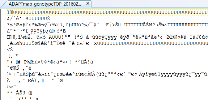
Figure 6.4: The .bed file opened with a text editor
This is because the genotypes are coded in a so-called binary format. This not just takes a very small hard disk space, but it is processed quicker by the computer since it's already translated from human-readable to a machine-readable format. Of course, quite often it is very useful to check out the individual genotypes, so to have them in a text format is required. The non-binary file format for the genotype is stored in the so-called ped and map files. These are also some very well-known (I dare to say iconic) file formats and widely used in various programs.
And how to get these files? It will be your task in your first actual use of the PLINK program. But don't worry! I will help you.
6.4 Excercise
Before you move on to the next section it is very useful to challenge yourself and your understanding of the topic that was just discussed. For this time, download this genotype dataset from Dryad, connected to the Decker et al.(2014) paper.
Questions to answer:
How many animals were genotyped?
How many SNPs are available in the data set?
After you have your answer, head over to my YouTube channel to find the solution with some bonus content on this issue.
If the embedded video does not start, click it again to "Watch on YouTube". Direct link: https://www.youtube.com/watch?v=vZyf5aXlB-k