Chapter 8 Genotype data quality control
Learning outcomes: At the end of this chapter you will be able to filter out low-quality genotypes from your data using PLINK.
At this point, you already know how the genomic data looks like (Genotype files in practice chapter) and how to process it with PLINK (Your first PLINK tutorial chapter). So it is reasonable to assume that you want to do some kind of real analysis at some point. But here I am to tell you: Do not rush it!
Before you do any kind of analysis, you need to check the quality of your genotype data and delete the sketchy parts. The good old saying "Garbage in, garbage out." is valid also here, so you want to avoid this by doing quality control (QC). This chapter will tell you how, why, and when to do certain moves.
We will start with a toy example and then move to the implementation in PLINK.
8.1 A toy example
In this example, we will consider a data set with five individuals each of them genotyped for five SNPs. The genotypes themselves are in numerical coding, 11 and 22 being the two homozygous, 12 the heterozygous, and 00 coded as missing.
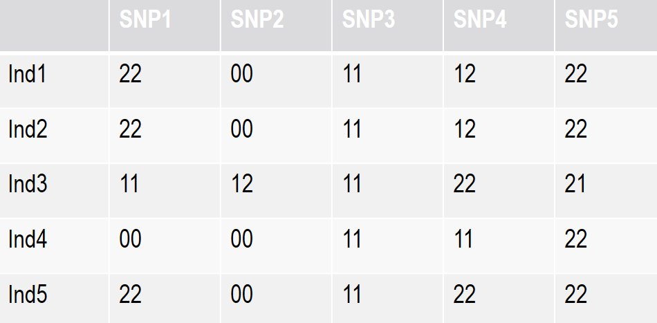
Figure 8.1: A small scale example for genotype quality control
8.1.1 Missingness per SNP
Overall, the SNP genotyping platform is very reliable and delivers stable results when it comes to determining genotypes. Of course, it is not flawless. One of the most frequent problems is that some of the SNPs are just not well genotyped in the entire population. These should be removed to improve the overall data quality.
Of course, we can not remove every SNP that has any missing value, as this way we would purge the entirety of our data. As a comproimse, we define thresholds instead. The funny thing about these thresholds is that no rule would firmly set which ones to use. So you are free to define them as long as you remain within "reasonable" bounds. To find out what "reasonable" means, it is perhaps a good idea to study the literature for your species of interest.
In this toy example, we will go with a 20% threshold. In other words, we would delete any SNP with more than 20% missing SNPs. In our case, SNP2 would be deleted.
8.1.2 Missingness per individual
The reliability of SNP chips is also high when it comes to individual genotypes. In some cases, however, some of the individuals contain a large number of missing SNPs. The reason could be low DNA sample quality, wrong chip type used (e.g. cattle chip for deer samples), or other technical issues. Regardless of the reason, you should delete the worst offenders from your data set, not to compromise the overall quality of your results.
In our toy example, we go with a 30% threshold, which means that individual 4 is deleted.
An interesting question is the follow-up of the quality control steps. If we would define a more conventional 10% threshold in our toy example, this would remove all genotypes. If we implement the filtering first by SNP (removing the problematic SNP2), and the filtering for individuals just after that, we are in much better shape.
8.1.3 Minor allele frequency
You can compute the proportion of any allele in any SNP based on the set of genotype data you have. For example in SNP4 we have five genotypes with a total of 10 alleles, four of them are Allele1 (40% or 0.4), and six of them Allele2 (60% or 0.6).
The Allele occurring less frequently will be the so-called minor allele, and the proportion of its occurrence called minor allele frequency (MAF). In the case of SNP4, the Allele1 is the minor allele, with a frequency of 0.4.
Limitations on the minor allele frequencies are done similarly as previously. You just define a number and every SNP with MAF below this number gets deleted. If you want to get rid only of the fixed SNPs, you specify a MAF threshold of 0.
8.1.4 Adherence to Hardy-Weinberg distribution
The quality control based on Hardy-Weinberg (H-W) distribution is a bit trickier to explain. You might know the definition of the Hardy-Weinberg rule from population genetics which states that genetic variation (thus allele and genotype frequencies) in a population will remain constant unless certain disturbing elements are introduced. This also means that when we know the allele frequencies for p and q, the genotype frequencies will be defined as p2, 2pq, and q2.
A more detailed example on Hardy-Weinberg limitation
Let's say the frequency of allele A (p in the equation)is 0.4, and that of allele B (q in the equation) is 0.6. This means for the H-W scenario the genotype frequencies will be 0.16 for AA, 0.48 for AB, and 0.36 for BB. This also means that in a population of e.g. 1000 individuals with the mentioned allele frequencies we expect to see 160 AA, 480 AB, and 360 BB individuals. Of course, we rarely see exact H-W distributions in real populations. The question then becomes, what is the extent of the difference between the expected H-W proportions in each SNP, and the observed proportions in the reality?
The way to provide a threshold to exclude unwanted SNPs is via a p-value threshold. If the expected and observed genotype frequencies are "equal" based on an equilibrium exact test with the significance (p-value) you provide, the SNP is kept during the quality control. If there are large differences between the expected and observed frequencies, the SNP is deleted.
From personal experience, I know that referring to p-values as "high" or "low" could be confusing, as you can never be too certain if this is meant as the numerical value or the strictness level (with lower p-values are being more strict). So to be very straightforward: you delete much more SNPs (i.e. you do a stricter QC) with the H-W significance threshold of e.g. 0.001 than if you set this to e.g. 0.000000001.
8.2 How QC works in PLINK
The implementation of the quality control steps in PLINK is easy. Remember the line in Your first PLINK tutorial? All you need to do is to include the corresponding PLINK options to that line with the quality control parameters of your choice. You could of course search for them on the options list I showed you, but for now, I am going to give you a head start:
Missingness per SNP: --geno value
Missingness per individual: --mind value
Minor allele frequency: --maf value
Hardy-Weinberg threshold: --hwe value
An additional very frequently used option is --autosome. By including this option you automatically keep only SNPs on the autosomal chromosomes. So any unplaced SNPs or those on the sex chromosomes get removed.
Caution! The --maf option is not considered in founder animals, i.e. those with unknown parents. Please note that the parentage information is many times skipped from data sets out of convenience or because it is not available. To include such animals in the quality control, use the --nonfounders option in your script.
8.3 Exceptions from SNP quality control
When NOT to include certain parameters into the QC?
Depending on the analysis you want to perform, you might not want to include some of the parameters mentioned above. This is because by doing so, you might be deleting the very results you are looking for.
Let me explain...
For example, you want to do anything with runs of homozygosity (ROH) - to look for long homozygous segments, that could be also fixed in the population. Implementing any kind of MAF filtering would get rid of fixed or highly homozygous SNPs. In the next step of your analysis, you would then proceed to look for fixed or highly homozygous regions on the genome... Ehm... You see how this went wrong, right?
Another example is if you are interested to look for previously unmapped disorders via the approach called "missing homozygosity". This method is based on the fact that you see much less homozygous genotypes for a certain allele compared to the expectations. The reason for the apparent lack of homozygotes might be because these alleles are in fact deleterious recessives. So any individual having them in homozygous form dies before it gets a chance to be genotyped. Of course, this also means that there will be an imbalance between observed and expected genotypes. The very result you are looking for! In case you apply the Hardy-Weinberg filtering however, you delete these from your records in the quality control step, as they are out of HWE expectations...
So I hope you get the picture... Quality control is necessary, but a cautious implementation is advised.
8.4 Exercise
You made it to the end! Congratulations!
You might have noticed that I did not give a full PLINK line on how to implement the QC to your existing script. That is because I want YOU to do it! That's right! This way you will reinforce your knowledge on QC and get a bit more practice with the implementation.
Take the PLINK line from your first PLINK tutorial with the ADAPmap data, and extend it with the following QC parameters:
Missingness per SNP: 0.1; Missingness per individual: 0.1; Minor allele frequency: 0.05
The questions are: What was the number of animals and SNPs before and after quality control? How many individuals and SNPs were removed due to the different criteria? Optional: See what happens if you include also a Hardy-Weinberg threshold: 0.0000001
As always, you can compare your solution with mine. In the video link below I discuss this exercise.
If the embedded video does not start, click it again to "Watch on YouTube". Direct link: https://www.youtube.com/watch?v=QR80Y0Xhrg4